7. Advanced Calculation and Statistical Methods#
Regridding#
Different datasets usually have different time and grid resolutions. Sometimes we need to use different datasets with the same resolution, so we need to regrid the A grid onto the B grid resolution. The simplest way to do this with xarray is using xr.interp. The default interpolation method of the xr.interp function is linear interpolation.
Example 1: The horizontal resolution of GPCP rainfall data is 2.5˚, and the horizontal resolution of OLR is 1˚. Now we will regrid the OLR data to the GPCP resolution.
import xarray as xr
lats = -20
latn =  30
lon1 =  79
lon2 = 161

pcp_ds = xr.open_dataset('data/gpcp_precip_1979-2019.pentad.nc')
pcp = pcp_ds.sel(lat=slice(latn,lats), lon=slice(lon1,lon2)).data
olr_ds = xr.open_dataset('data/olr.nc')
olr = olr_ds.sel(lat=slice(lats,latn), lon=slice(lon1,lon2)).olr

olr_rmp = olr.interp(lon=pcp.lon, lat=pcp.lat)   # Specify the target grid info to the `interp` method.
olr_rmp
<xarray.DataArray 'olr' (time: 8760, lat: 20, lon: 32)> Size: 22MB
array([[[210.37125, 199.29874, 197.44077, ..., 268.05853, 268.25916,
         266.9823 ],
        [204.61313, 213.93433, 230.92719, ..., 284.24072, 282.60632,
         278.35385],
        [236.69272, 247.62692, 259.35587, ..., 294.86554, 292.45862,
         292.01804],
        ...,
        [297.27472, 302.5027 , 305.18634, ..., 193.11395, 206.42505,
         197.59212],
        [291.31464, 291.11176, 298.43726, ..., 155.4393 , 146.58469,
         162.1478 ],
        [286.89136, 290.6887 , 291.20618, ..., 171.58977, 183.45123,
         195.39035]],

       [[259.8478 , 225.8486 , 211.98647, ..., 269.50348, 269.39746,
         272.64   ],
        [276.39136, 272.1738 , 268.95856, ..., 291.94778, 289.79297,
         284.37097],
        [260.77368, 265.89886, 275.41898, ..., 301.7583 , 299.66028,
         292.9348 ],
...
        [289.9028 , 281.8377 , 285.37466, ..., 169.81645, 173.29109,
         213.98285],
        [286.0285 , 282.36426, 284.31454, ..., 111.96492, 154.03249,
         224.03793],
        [290.05353, 295.02466, 291.87067, ..., 125.69296, 153.77583,
         191.87067]],

       [[240.00652, 211.87251, 198.56546, ..., 264.23984, 258.3333 ,
         255.25803],
        [224.23218, 243.02698, 246.38681, ..., 279.6334 , 274.43097,
         277.21472],
        [234.04726, 253.98969, 263.0449 , ..., 289.64203, 291.71185,
         293.91864],
        ...,
        [286.8454 , 287.29822, 284.08643, ..., 165.07278, 165.68568,
         180.77968],
        [291.43097, 289.64923, 295.36426, ..., 178.16243, 158.17258,
         182.52911],
        [294.91678, 297.96875, 296.73392, ..., 174.35318, 157.13422,
         152.69089]]], dtype=float32)
Coordinates:
  * time     (time) datetime64[ns] 70kB 1998-01-01 1998-01-02 ... 2021-12-31
  * lon      (lon) float32 128B 81.25 83.75 86.25 88.75 ... 153.8 156.2 158.8
  * lat      (lat) float32 80B 28.75 26.25 23.75 21.25 ... -13.75 -16.25 -18.75
Attributes:
    standard_name:  toa_outgoing_longwave_flux
    long_name:      NOAA Climate Data Record of Daily Mean Upward Longwave Fl...
    units:          W m-2
cell_methods: time: mean area: meanHowever, sometimes linear interpolation is not the best way to regrid. For example, rainfall need to stay mass conservation after regridding, therefore conservative regridding is required. Here we introduce xesmf library to do this.
Example 2: Regrid the GPCP data to the OLR resolution.
import xesmf as xe

# Set the grid information
grid_olr  = xr.Dataset({'lat':olr.lat, 'lon':olr.lon})
grid_gpcp = xr.Dataset({'lat':pcp.lat, 'lon':pcp.lon})
# ds_in: the input grid info;
# ds_out: the output grid info
regridder = xe.Regridder(ds_in=grid_gpcp , ds_out=grid_olr, method="conservative_normed")
pcp_rg = regridder(pcp,keep_attrs=True)
---------------------------------------------------------------------------
KeyError                                  Traceback (most recent call last)
Cell In[2], line 1
----> 1 import xesmf as xe
      3 # Set the grid information
      4 grid_olr  = xr.Dataset({'lat':olr.lat, 'lon':olr.lon})

File /data/wtsai/micromamba/p3t/lib/python3.10/site-packages/xesmf/__init__.py:3
      1 # flake8: noqa
----> 3 from . import data, util
      4 from .frontend import Regridder, SpatialAverager
      6 try:

File /data/wtsai/micromamba/p3t/lib/python3.10/site-packages/xesmf/util.py:8
      5 from shapely.geometry import MultiPolygon, Polygon
      7 try:
----> 8     import esmpy as ESMF
      9 except ImportError:
     10     import ESMF

File /data/wtsai/micromamba/p3t/lib/python3.10/site-packages/esmpy/__init__.py:106
    104 __requires_python__ = msg["Requires-Python"]
    105 # these don't seem to work with setuptools pyproject.toml
--> 106 __author__ = msg["Author"]
    107 __homepage__ = msg["Home-page"]
    108 __obsoletes__ = msg["obsoletes"]

File /data/wtsai/micromamba/p3t/lib/python3.10/site-packages/importlib_metadata/_adapters.py:101, in Message.__getitem__(self, item)
     99 res = super().__getitem__(item)
    100 if res is None:
--> 101     raise KeyError(item)
    102 return res

KeyError: 'Author'
Coarsen Grid Resolution#
We can also coarsen the grid resolution using xarray.DataArray.coarsen.
Example 3: Convert daily OLR data to pentad mean. (This means to coarsen the grid resolution from daily to pentad.)
olr_noleap = olr.sel(time=~((olr.time.dt.month == 2) & (olr.time.dt.day == 29))) # Remove the leap days.
olr_ptd = (olr_noleap.coarsen(time=5,
                              coord_func={"time": "min"})  # Set the coordinate values to the min. of the 5-day period
                                                           # (or the pentad start day)
                     .mean())
olr_ptd
<xarray.DataArray 'olr' (time: 1752, lat: 50, lon: 82)> Size: 29MB
array([[[284.27383, 285.73615, 288.25266, ..., 231.88799, 241.6569 ,
         249.84024],
        [286.65228, 288.0508 , 288.27435, ..., 215.95383, 230.82944,
         246.1481 ],
        [290.7838 , 290.2586 , 287.82904, ..., 198.27681, 214.98921,
         225.9622 ],
        ...,
        [247.29614, 246.06245, 247.9498 , ..., 279.0298 , 277.99088,
         276.57684],
        [244.55948, 242.81021, 239.57669, ..., 273.2099 , 271.63373,
         270.99365],
        [236.1903 , 229.96805, 221.43008, ..., 266.5147 , 266.81476,
         266.7093 ]],

       [[257.097  , 249.0689 , 260.7727 , ..., 251.24785, 258.4394 ,
         267.57504],
        [265.49664, 263.9062 , 270.4431 , ..., 237.29636, 248.2174 ,
         250.10226],
        [261.7508 , 266.22888, 276.74783, ..., 222.4416 , 235.64157,
         227.53247],
...
        [246.52588, 246.06046, 249.06099, ..., 256.54034, 259.21564,
         260.40427],
        [244.2377 , 247.02632, 246.57185, ..., 258.28464, 255.90445,
         257.71054],
        [237.54703, 235.23251, 224.96394, ..., 255.28891, 253.66435,
         255.53586]],

       [[286.864  , 287.83688, 290.30945, ..., 194.66502, 212.79057,
         210.36748],
        [288.31   , 288.92453, 290.12537, ..., 204.64694, 225.9674 ,
         223.37724],
        [284.80383, 288.20563, 289.7766 , ..., 215.14029, 236.13554,
         232.43852],
        ...,
        [236.44717, 236.95544, 234.64787, ..., 268.50082, 268.91937,
         267.25333],
        [235.04623, 231.87952, 229.08992, ..., 267.69647, 267.49542,
         266.0851 ],
        [233.44182, 225.93411, 211.10928, ..., 268.23108, 265.9177 ,
         264.84662]]], dtype=float32)
Coordinates:
  * time     (time) datetime64[ns] 14kB 1998-01-01 1998-01-06 ... 2021-12-27
  * lon      (lon) float32 328B 79.5 80.5 81.5 82.5 ... 157.5 158.5 159.5 160.5
  * lat      (lat) float32 200B -19.5 -18.5 -17.5 -16.5 ... 26.5 27.5 28.5 29.5
Attributes:
    standard_name:  toa_outgoing_longwave_flux
    long_name:      NOAA Climate Data Record of Daily Mean Upward Longwave Fl...
    units:          W m-2
cell_methods: time: mean area: meanWe actually average the time coordinate over every 5 days. The default setting of coord_func is mean, where the coarsened coordinate will be set as the date of the 5-day average (e.g., 1998-01-03, 1998-01-08, 1998-01-13, …). Other options include min (the start date of the pentad) or max (the end date of the pentad).
Note
xarray.DataArray.resample seems to have the same function. From API reference,
The resampled dimension must be a datetime-like coordinate.
First of all, coarsen can be operated on any coordinate, whereas resample can only be operated on a datetime-like coordinate. Additionally, we cannot skip leap days since the resample frequency is entirely based on the datetime object (See this StackOverflow post). Therefore, olr_ptd = olr_noleap.resample(time='5D') will still consider Feb. 29 even if we exclude leap days in the data.
Running Mean#
Running mean is often applied to remove or smooth out high-frequency variability. For example, Takaya and Nakamura (2001, JAS) used a 10-day running mean to remove high-frequency variability within a 10-day period before calculating the Rossby wave activity flux. When calculating Realtime Multivariate MJO (RMM) index, Gottschalck et al. (2010, BAMS) removed interannual variability by subtracting the 120-day running mean before performing the combined EOF analysis. In xarray, we can use the xarray.DataArray.rolling method to calculate the running mean.
olr_3p_runave = (olr_ptd.rolling(time=3,
                                 center=False)
                        .mean()
                        .dropna('time'))
olr_3p_runave
<xarray.DataArray 'olr' (time: 1750, lat: 50, lon: 82)> Size: 29MB
array([[[267.31717, 266.99036, 270.8208 , ..., 247.27075, 253.0514 ,
         259.74832],
        [272.3418 , 271.4567 , 273.70862, ..., 235.08034, 243.3069 ,
         250.87163],
        [270.9473 , 272.3905 , 274.61237, ..., 223.71478, 231.73334,
         233.63165],
        ...,
        [242.48238, 243.38196, 246.27788, ..., 271.20895, 271.14975,
         270.8715 ],
        [239.12952, 239.81575, 242.67973, ..., 266.25696, 266.15314,
         266.28625],
        [234.36653, 231.1346 , 223.61658, ..., 259.56998, 260.0516 ,
         260.38214]],

       [[264.36322, 261.904  , 264.3725 , ..., 238.1038 , 241.9434 ,
         249.87357],
        [269.2213 , 267.343  , 269.49976, ..., 232.33305, 237.68199,
         241.17148],
        [266.89197, 267.56128, 270.72424, ..., 229.26079, 234.51195,
         233.8206 ],
...
        [258.01865, 258.54132, 260.59457, ..., 265.62262, 266.46997,
         267.72852],
        [254.52092, 255.43341, 253.74515, ..., 262.07703, 262.12787,
         264.36252],
        [249.05486, 243.50095, 230.53357, ..., 257.8312 , 259.1329 ,
         259.55786]],

       [[285.45612, 286.57214, 287.6652 , ..., 247.677  , 257.28473,
         259.3609 ],
        [288.13184, 288.3128 , 289.0145 , ..., 255.27068, 264.8253 ,
         264.77902],
        [288.0848 , 289.45697, 289.93057, ..., 261.4938 , 269.81818,
         268.2691 ],
        ...,
        [248.90976, 249.10083, 250.33572, ..., 262.9018 , 263.4146 ,
         263.58185],
        [247.00436, 247.02068, 245.05011, ..., 261.76514, 261.24374,
         261.8905 ],
        [243.24814, 237.90851, 224.16135, ..., 258.3669 , 257.77066,
         257.97882]]], dtype=float32)
Coordinates:
  * time     (time) datetime64[ns] 14kB 1998-01-11 1998-01-16 ... 2021-12-27
  * lon      (lon) float32 328B 79.5 80.5 81.5 82.5 ... 157.5 158.5 159.5 160.5
  * lat      (lat) float32 200B -19.5 -18.5 -17.5 -16.5 ... 26.5 27.5 28.5 29.5
Attributes:
    standard_name:  toa_outgoing_longwave_flux
    long_name:      NOAA Climate Data Record of Daily Mean Upward Longwave Fl...
    units:          W m-2
cell_methods: time: mean area: meanWe can use dropna() to remove missing values.
Correlation Map#
We can calculate the correlation coefficient between two DataArrays along a specific coordinate.
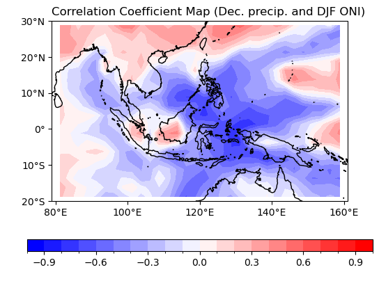
Example 4: Plot the correlation coefficient map between NDJ Oceanic Niño Index (ONI) and December rainfall.
Step 1: Retrieve GPCP monthly mean rainfall in December. (Choose all data in December, then group and average by each year with groupby.)
pcp_dec = (pcp.sel(time=pcp.time.dt.month.isin([12]))
              .groupby('time.year')
              .mean("time"))
pcp_dec
<xarray.DataArray 'data' (year: 41, lat: 20, lon: 32)> Size: 105kB
array([[[1.0133333e+00, 9.1833329e-01, 7.9833335e-01, ...,
         3.6333334e+00, 2.7116668e+00, 2.5383332e+00],
        [2.0333333e-01, 4.2833331e-01, 2.5000000e-01, ...,
         2.4483333e+00, 2.3216665e+00, 1.7766665e+00],
        [5.4999996e-02, 1.3666667e-01, 1.5833335e-01, ...,
         2.2033336e+00, 1.8683332e+00, 1.2850000e+00],
        ...,
        [1.1466666e+00, 1.4949999e+00, 1.8333334e+00, ...,
         3.6483333e+00, 4.2433333e+00, 2.9916668e+00],
        [7.1833330e-01, 1.3866667e+00, 1.4466667e+00, ...,
         4.0750003e+00, 3.2466669e+00, 2.8599999e+00],
        [3.9666665e-01, 8.2333332e-01, 1.1883334e+00, ...,
         2.9016666e+00, 2.7083333e+00, 1.7416667e+00]],

       [[4.6500000e-01, 2.8333333e-01, 3.4333333e-01, ...,
         3.8716667e+00, 3.8799999e+00, 3.4633334e+00],
        [6.0833335e-01, 1.7000000e-01, 1.4666666e-01, ...,
         3.9750001e+00, 3.6300001e+00, 3.1483333e+00],
        [1.2800001e+00, 3.2166669e-01, 1.2000000e-01, ...,
         2.4466667e+00, 2.1550000e+00, 1.1616668e+00],
...
        [7.9235015e+00, 7.0794005e+00, 5.7172127e+00, ...,
         9.7668800e+00, 1.0939357e+01, 1.0846936e+01],
        [9.5492640e+00, 7.4848499e+00, 3.3095343e+00, ...,
         1.2228072e+01, 1.2528176e+01, 1.1302447e+01],
        [7.2531962e+00, 5.3915715e+00, 2.0546637e+00, ...,
         1.0486613e+01, 1.3482674e+01, 1.1387763e+01]],

       [[2.0096309e+00, 1.1509016e+00, 4.8980752e-01, ...,
         2.0202532e+00, 2.7056713e+00, 2.6676538e+00],
        [1.2896461e+00, 1.1470729e+00, 2.6983759e-01, ...,
         1.3239046e+00, 1.6525987e+00, 1.6284056e+00],
        [8.9463830e-01, 3.9747801e-01, 1.5476857e-01, ...,
         1.1533502e+00, 1.1403440e+00, 9.9328095e-01],
        ...,
        [1.2956619e+00, 6.6536534e-01, 5.8920252e-01, ...,
         4.1320643e+00, 4.3791137e+00, 4.1250496e+00],
        [1.7519032e+00, 1.2151116e+00, 9.6764684e-01, ...,
         5.1612849e+00, 5.1797566e+00, 2.8651981e+00],
        [3.1523111e+00, 2.0467207e+00, 1.0773114e+00, ...,
         3.6295269e+00, 4.3244128e+00, 2.4604805e+00]]], dtype=float32)
Coordinates:
  * lon      (lon) float32 128B 81.25 83.75 86.25 88.75 ... 153.8 156.2 158.8
  * lat      (lat) float32 80B 28.75 26.25 23.75 21.25 ... -13.75 -16.25 -18.75
  * year     (year) int64 328B 1979 1980 1981 1982 1983 ... 2016 2017 2018 2019
Attributes:
    long_name:  GPCP pentad precipitation (mm/day)
units: mm/dayStep 2: Create the DataArray for NDJ ONI.
oni_ndj = xr.DataArray(
                       data=[0.6, 0.0, -0.1, 2.2, -0.9, -1.1, -0.4, 1.2, 1.1, -1.8, -0.1, 0.4,
                             1.5, -0.1, 0.1, 1.1, -1.0, -0.5, 2.4, -1.6, -1.7, -0.7,
                             -0.3, 1.1, 0.4, 0.7, -0.8, 0.9, -1.6, -0.7, 1.6, -1.6,
                             -1.0, -0.2, -0.3, 0.7, 2.6, -0.6, -1.0, 0.8, 0.5],
                       dims='year',
                       coords=dict(year=pcp_dec.year)
                       )
oni_ndj
<xarray.DataArray (year: 41)> Size: 328B
array([ 0.6,  0. , -0.1,  2.2, -0.9, -1.1, -0.4,  1.2,  1.1, -1.8, -0.1,
        0.4,  1.5, -0.1,  0.1,  1.1, -1. , -0.5,  2.4, -1.6, -1.7, -0.7,
       -0.3,  1.1,  0.4,  0.7, -0.8,  0.9, -1.6, -0.7,  1.6, -1.6, -1. ,
       -0.2, -0.3,  0.7,  2.6, -0.6, -1. ,  0.8,  0.5])
Coordinates:
* year (year) int64 328B 1979 1980 1981 1982 1983 ... 2016 2017 2018 2019Step 3: Calculate correlation coefficient with xr.corr.
corr = xr.corr(pcp_dec,oni_ndj,dim='year')
corr
<xarray.DataArray (lat: 20, lon: 32)> Size: 5kB
array([[ 3.62929452e-01,  3.42366940e-01,  1.36141381e-01,
         2.86181877e-01,  1.81635011e-01,  1.49191935e-01,
         2.91984738e-01,  4.77790090e-01,  4.72934980e-01,
         2.59950214e-01,  3.45925708e-01,  3.45836394e-01,
         2.41839291e-01,  3.26920710e-01,  3.12002374e-01,
         2.78955901e-01,  2.83943380e-01,  3.95803478e-01,
         4.20742082e-01,  4.71375054e-01,  5.46175408e-01,
         4.34086513e-01,  3.36992606e-01,  2.34458541e-01,
         3.30061218e-01,  2.83089068e-01,  6.62670164e-02,
        -6.41038383e-02, -8.02357126e-02, -1.32435603e-01,
        -6.14116577e-02, -3.57627814e-01],
       [ 3.83909992e-01,  3.03894569e-01,  2.37785616e-01,
         2.14941985e-01,  1.29919746e-01,  9.02064270e-02,
         1.65142441e-01,  2.02511225e-01,  2.68816760e-01,
         1.56273306e-01,  2.46169172e-01,  3.13843032e-01,
         3.71282408e-01,  3.76425080e-01,  3.56976471e-01,
         3.31840158e-01,  1.84695348e-01,  4.19843103e-01,
         4.71277802e-01,  4.27318315e-01,  3.51365941e-01,
         2.37002936e-01,  2.34139483e-01,  2.04142669e-01,
         1.27191143e-01, -7.16084696e-02, -1.17030947e-01,
...
        -1.63141768e-01,  2.02073897e-02,  8.64961746e-02,
        -6.46166022e-02, -1.30967877e-01, -1.11179142e-01,
        -2.19488532e-01, -3.89394358e-01, -5.41138822e-01,
        -5.55411026e-01, -4.62892792e-01, -3.87886292e-01,
        -2.86447705e-01, -1.87858258e-01, -4.88526454e-02,
        -6.03390847e-02, -5.92937090e-02, -1.09022036e-02,
        -1.62940957e-01, -1.06521335e-01, -1.63654755e-01,
        -2.66138359e-01, -3.63495708e-01, -3.56191141e-01,
        -3.43018577e-01, -4.02329768e-01],
       [ 2.18229674e-01,  1.50764053e-01,  4.34983986e-02,
        -2.31485323e-02, -1.24680824e-01, -2.82829682e-01,
        -2.27022130e-01, -1.80625258e-01, -6.68313221e-02,
        -1.22718863e-01, -7.70160205e-02, -1.92838402e-01,
        -2.63437027e-01, -4.77678622e-01, -6.13706400e-01,
        -5.25689477e-01, -3.34162312e-01, -3.46265756e-01,
        -2.73299118e-01, -3.36175549e-01, -1.75612517e-01,
        -7.18667375e-02, -2.45879325e-02,  2.50092056e-03,
        -1.46619847e-01, -7.41479127e-02, -3.23609552e-02,
        -1.90437815e-01, -2.59385858e-01, -3.08636758e-01,
        -2.93624427e-01, -3.09437346e-01]])
Coordinates:
  * lon      (lon) float32 128B 81.25 83.75 86.25 88.75 ... 153.8 156.2 158.8
* lat (lat) float32 80B 28.75 26.25 23.75 21.25 ... -13.75 -16.25 -18.75Step 4: Plot result.
import numpy as np
from cartopy import crs as ccrs
from cartopy.mpl.gridliner import LONGITUDE_FORMATTER, LATITUDE_FORMATTER
import matplotlib as mpl
from matplotlib import pyplot as plt
mpl.rcParams['figure.dpi'] = 100

proj = ccrs.PlateCarree()
fig, ax = plt.subplots(1,1,subplot_kw={'projection':proj})

clevs = np.arange(170,350,20)

corrPlot = (corr.plot.contourf("lon", "lat",
                               ax=ax,
                               levels=np.arange(-1,1.1,0.1),
                               cmap='bwr',
                               add_colorbar=True,
                               extend='neither',
                               cbar_kwargs={'orientation': 'horizontal', 'aspect': 30, 'label': ' '}) #設定color bar
                               )
ax.set_extent([lon1,lon2,lats,latn],crs=proj)
ax.set_xticks(np.arange(80,180,20), crs=proj)
ax.set_yticks(np.arange(-20,40,10), crs=proj)
lon_formatter = LONGITUDE_FORMATTER
lat_formatter = LATITUDE_FORMATTER
ax.xaxis.set_major_formatter(lon_formatter)
ax.yaxis.set_major_formatter(lat_formatter)
ax.coastlines()
ax.set_ylabel(' ')             # 設定坐標軸名稱。
ax.set_xlabel(' ')
ax.set_title("Correlation Coefficient Map (Dec. precip. and DJF ONI)", loc='left')
plt.show()
Conditional Control with where#
We can filter and select data using specified conditions. The usage is
xarray.where(cond, x, y, keep_attrs=None)
When True, return values from x, otherwise returns values from y.
Example 4: Plot the mean sea level pressure (MSLP) map in December 2021, excluding regions with altitudes higher than 3000 meters.
Step 1: Read data: MSLP and topography.
lats=0
latn=60

topo_ds = xr.open_dataset('data/etopo5.nc')
mslp_ds = xr.open_dataset('data/mslp.2021.nc')
topo = topo_ds.sel(Y=slice(lats,latn),
                   X=slice(lon1,lon2)).bath
mslp = mslp_ds.sel(time=slice('2021-12-01','2021-12-31'),
                   lat=slice(latn,lats),
                   lon=slice(lon1,lon2)).mslp
mslp = mslp/100. # Convert to hPa.
In this example, the grid resolution of the conditional array (topo) and the mslp array should be the same so that xarray can look for corresponding grids that satisfy the condition. Therefore, we need to regrid the data first.
topo_rmp = topo.interp(X=mslp.lon, Y=mslp.lat).drop_vars(['X','Y'])
Then set the condition with where:
mslp_mean = mslp.mean('time')
mslp_mask = xr.where(topo_rmp<=3000,mslp_mean,np.nan)
The condition is topo <= 3000. The False values (those that don’t satisfy the criteria) will be set as NaN. The True values will be preserved.
proj = ccrs.PlateCarree()
fig, ax = plt.subplots(1,1,subplot_kw={'projection':proj})

# Plotting
Plot = mslp_mask.plot.contourf("lon", "lat",
                                ax=ax,
                                levels=np.arange(986,1048,8),
                                cmap='coolwarm',
                                add_colorbar=True,
                                extend='both',
                                cbar_kwargs={'orientation': 'horizontal', 'aspect': 30, 'label': '[hPa]'}) #設定color bar
ax.set_extent([lon1,lon2,lats,latn],crs=proj)
ax.set_xticks(np.arange(80,180,20), crs=proj)
ax.set_yticks(np.arange(0,70,10), crs=proj)
lon_formatter = LONGITUDE_FORMATTER
lat_formatter = LATITUDE_FORMATTER
ax.xaxis.set_major_formatter(lon_formatter)
ax.yaxis.set_major_formatter(lat_formatter)
ax.coastlines()
ax.set_ylabel(' ')
ax.set_xlabel(' ')
ax.set_title("MSLP, Dec. 2021", loc='left')

plt.show()
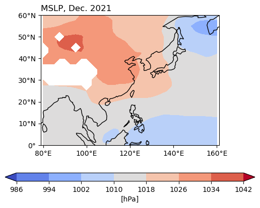
Regions exceeding 3000 meters in altitude are set as NaN, so no values are plotted over these areas.
Calculate Relative Vorticity and Divergence#
Simple statistics can be done with xarray’s methods. When it comes to meteorological variables, we can use the MetPy library. MetPy supports xarray, which means that we can apply DataArray to MetPy functions. Below is an example to calculate relative vorticity using metpy.calc.vorticity.
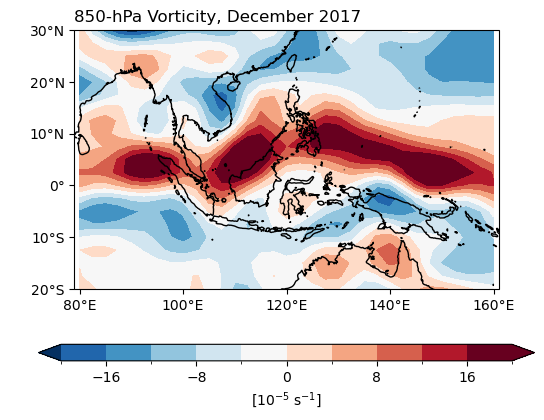
Example 5: Calculate relative vorticity at the 850-hPa level in December 2017.
Step 1: Read data and select the spatial and temporal ranges.
latn = 30
lats = -20

uds = xr.open_dataset('data/ncep_r2_uv850/u850.2017.nc')
vds = xr.open_dataset('data/ncep_r2_uv850/v850.2017.nc')
u = uds.sel(time=slice('2017-12-01','2017-12-31'),
            level=850,
            lat=slice(latn,lats),
            lon=slice(lon1,lon2)).uwnd
v = vds.sel(time=slice('2017-12-01','2017-12-31'),
            level=850,
            lat=slice(latn,lats),
            lon=slice(lon1,lon2)).vwnd
Step 2: Calculate relative vorticity. Ensure that the vorticity function requires units for the wind field. Import metpy.units and attach it to the wind variables.
import metpy.calc as mpcalc
from metpy.units import units
vor = mpcalc.vorticity(u*units('m/s'), v*units('m/s'))
vorm = vor.mean(axis=0)
vorm
<xarray.DataArray (lat: 21, lon: 33)> Size: 6kB
<Quantity([[ 2.27227035e-06 -6.35822645e-06 -1.46749070e-05 -2.08053115e-05
  -2.30204190e-05 -2.14179636e-05 -1.73882539e-05 -1.29046760e-05
  -9.84929500e-06 -9.54206099e-06 -1.12507049e-05 -1.23807539e-05
  -1.01248504e-05 -4.97617877e-06 -9.28601335e-07 -2.13257232e-06
  -8.04519296e-06 -1.36745794e-05 -1.37081362e-05 -8.49913312e-06
  -2.77764758e-06 -1.18851542e-06 -3.59719131e-06 -6.00788240e-06
  -5.68558831e-06 -3.57765352e-06 -2.98596786e-06 -5.61280440e-06
  -9.78352706e-06 -1.28709753e-05 -1.36409031e-05 -1.30405734e-05
  -1.21284570e-05]
 [ 1.59641488e-06  1.27951490e-07 -2.96147587e-06 -6.09627077e-06
  -7.14075885e-06 -6.30349598e-06 -5.16875042e-06 -4.56615673e-06
  -4.01070010e-06 -3.29133037e-06 -3.14996178e-06 -4.03313727e-06
  -5.06772766e-06 -5.30085544e-06 -5.33611754e-06 -7.06711890e-06
  -1.08910896e-05 -1.43131536e-05 -1.42338578e-05 -1.03047389e-05
  -5.71612173e-06 -3.96175474e-06 -5.53658936e-06 -7.88921794e-06
  -8.64479278e-06 -8.03751306e-06 -8.04710263e-06 -9.82336098e-06
  -1.24495122e-05 -1.41660453e-05 -1.44190610e-05 -1.42504704e-05
  -1.44654921e-05]
 [-2.25853323e-06  1.13172266e-06  2.50715062e-06  3.24109081e-06
   4.54796451e-06  5.22032636e-06  3.42384104e-06  8.61968466e-08
...
  -8.52059086e-06 -1.10716107e-05 -1.19881288e-05 -1.13950856e-05
  -9.98141214e-06]
 [ 3.40814844e-07 -1.87193747e-06 -2.55199434e-06 -1.83217317e-06
  -7.07930811e-07 -2.45485863e-07 -7.17219789e-07 -1.21135839e-06
  -6.77305687e-07  1.98063110e-07 -8.42058040e-07 -4.36596747e-06
  -7.21982209e-06 -6.11138032e-06 -2.24744337e-06  6.50249030e-08
  -5.85517420e-07 -8.93727851e-07  1.92617077e-06  5.34523983e-06
   4.91827661e-06  6.98802749e-07 -2.36916696e-06 -8.49899076e-07
   3.18171194e-06  5.20927594e-06  3.40469449e-06 -5.15668196e-07
  -4.15454945e-06 -6.51466556e-06 -7.57468620e-06 -7.70031620e-06
  -7.32678885e-06]
 [ 3.86059996e-06  4.83366406e-07 -1.67842807e-06 -2.14714011e-06
  -1.31075583e-06 -6.41593796e-07 -9.82999754e-07 -1.46979384e-06
  -7.01365099e-07  5.12796672e-07 -4.05116393e-07 -4.63963087e-06
  -8.87224706e-06 -8.92474419e-06 -4.83957896e-06 -1.08197146e-06
  -7.43141058e-07 -2.15767543e-06 -1.95926642e-06 -1.83126193e-07
  -9.75771821e-09 -3.08505634e-06 -6.80966442e-06 -7.53604087e-06
  -4.54671714e-06 -6.88500940e-08  3.41230334e-06  4.97175514e-06
   4.77222735e-06  3.07068630e-06  7.25767405e-07 -1.38476001e-06
  -2.89335635e-06]], '1 / second')>
Coordinates:
  * lon      (lon) float32 132B 80.0 82.5 85.0 87.5 ... 152.5 155.0 157.5 160.0
  * lat      (lat) float32 84B 30.0 27.5 25.0 22.5 ... -12.5 -15.0 -17.5 -20.0
level float32 4B 850.0In the preview of the variable vorm above, it includes information such as “Magnitude” and “Units”. A DataArray with unit information is referred to as a unit-aware array type. When applying this DataArray to follow-up calculations, the unit information will be preserved. However, some libraries and functions other than MetPy may not recognize unit-aware array types, leading to errors. In such cases, we can use .dequantify() to convert it to an ordinary DataArray, which is called a unit-naive array type.
vorm.metpy.dequantify()
<xarray.DataArray (lat: 21, lon: 33)> Size: 6kB
array([[ 2.27227035e-06, -6.35822645e-06, -1.46749070e-05,
        -2.08053115e-05, -2.30204190e-05, -2.14179636e-05,
        -1.73882539e-05, -1.29046760e-05, -9.84929500e-06,
        -9.54206099e-06, -1.12507049e-05, -1.23807539e-05,
        -1.01248504e-05, -4.97617877e-06, -9.28601335e-07,
        -2.13257232e-06, -8.04519296e-06, -1.36745794e-05,
        -1.37081362e-05, -8.49913312e-06, -2.77764758e-06,
        -1.18851542e-06, -3.59719131e-06, -6.00788240e-06,
        -5.68558831e-06, -3.57765352e-06, -2.98596786e-06,
        -5.61280440e-06, -9.78352706e-06, -1.28709753e-05,
        -1.36409031e-05, -1.30405734e-05, -1.21284570e-05],
       [ 1.59641488e-06,  1.27951490e-07, -2.96147587e-06,
        -6.09627077e-06, -7.14075885e-06, -6.30349598e-06,
        -5.16875042e-06, -4.56615673e-06, -4.01070010e-06,
        -3.29133037e-06, -3.14996178e-06, -4.03313727e-06,
        -5.06772766e-06, -5.30085544e-06, -5.33611754e-06,
        -7.06711890e-06, -1.08910896e-05, -1.43131536e-05,
        -1.42338578e-05, -1.03047389e-05, -5.71612173e-06,
        -3.96175474e-06, -5.53658936e-06, -7.88921794e-06,
        -8.64479278e-06, -8.03751306e-06, -8.04710263e-06,
...
        -7.17219789e-07, -1.21135839e-06, -6.77305687e-07,
         1.98063110e-07, -8.42058040e-07, -4.36596747e-06,
        -7.21982209e-06, -6.11138032e-06, -2.24744337e-06,
         6.50249030e-08, -5.85517420e-07, -8.93727851e-07,
         1.92617077e-06,  5.34523983e-06,  4.91827661e-06,
         6.98802749e-07, -2.36916696e-06, -8.49899076e-07,
         3.18171194e-06,  5.20927594e-06,  3.40469449e-06,
        -5.15668196e-07, -4.15454945e-06, -6.51466556e-06,
        -7.57468620e-06, -7.70031620e-06, -7.32678885e-06],
       [ 3.86059996e-06,  4.83366406e-07, -1.67842807e-06,
        -2.14714011e-06, -1.31075583e-06, -6.41593796e-07,
        -9.82999754e-07, -1.46979384e-06, -7.01365099e-07,
         5.12796672e-07, -4.05116393e-07, -4.63963087e-06,
        -8.87224706e-06, -8.92474419e-06, -4.83957896e-06,
        -1.08197146e-06, -7.43141058e-07, -2.15767543e-06,
        -1.95926642e-06, -1.83126193e-07, -9.75771821e-09,
        -3.08505634e-06, -6.80966442e-06, -7.53604087e-06,
        -4.54671714e-06, -6.88500940e-08,  3.41230334e-06,
         4.97175514e-06,  4.77222735e-06,  3.07068630e-06,
         7.25767405e-07, -1.38476001e-06, -2.89335635e-06]])
Coordinates:
  * lon      (lon) float32 132B 80.0 82.5 85.0 87.5 ... 152.5 155.0 157.5 160.0
  * lat      (lat) float32 84B 30.0 27.5 25.0 22.5 ... -12.5 -15.0 -17.5 -20.0
    level    float32 4B 850.0
Attributes:
units: 1 / secondThe unit will be converted to an ordinary text attribute.
This example highlights the advantages of using xarray.DataArray over numpy.array. With numpy.array, you would need to specify the number of latitude and longitude axes, as well as provide the longitude and latitude arrays. However, since the latitude and longitude labels and dimension names are already stored in the DataArray, you only need to provide the wind DataArrays. This makes the code significantly simpler.
Step 3: Plotting.
import cmaps

proj = ccrs.PlateCarree()
fig, ax = plt.subplots(1,1,subplot_kw={'projection':proj})

vorm = vorm * 10e5
vorPlot = (vorm.plot.contourf("lon", "lat",
                              ax=ax,
                              levels=np.arange(-20,24,4),
                              cmap=cmaps.CBR_coldhot,
                              add_colorbar=True,
                              extend='both',
                              cbar_kwargs={'orientation': 'horizontal', 'aspect': 30, 'label': r'[$10^{-5}$ s$^{-1}$]'}) #設定color bar
                              )
ax.set_extent([lon1,lon2,lats,latn],crs=proj)
ax.set_xticks(np.arange(80,180,20), crs=proj)
ax.set_yticks(np.arange(-20,40,10), crs=proj)
lon_formatter = LONGITUDE_FORMATTER
lat_formatter = LATITUDE_FORMATTER
ax.xaxis.set_major_formatter(lon_formatter)
ax.yaxis.set_major_formatter(lat_formatter)
ax.coastlines()

ax.set_title(' ')
ax.set_title('850-hPa Vorticity, December 2017', loc='left')
ax.set_ylabel(' ')             # 設定坐標軸名稱。
ax.set_xlabel(' ')
plt.show()
Exercise
Similar to Example 5, but for divergence (metpy.calc.divergence).
Empirical Orthogonal Functions (EOF)#
Can use eofs or xeofs libraries. For eofs, see instructions on their website.
from eofs.xarray import Eof
Set
solver = Eof(data_array)
solver includes several methods:
solver.eofs(): Calculates EOF modes. The neofs option specifies the number of modes to compute.solver.pcs(): Computes the time series of principal components.solver.varianceFraction(): Computes the ratio of variance explained by each EOF mode, indicating how much percentage of the original data variance each mode can explain.solver.reconstructedField(): Reconstructs the variable using EOF modes and their principal components.solver.projectField(): Projects the variable onto the EOF modes.
xeof library has more extensive EOF methods, such as multivariate EOF and rotate EOF. See instructions on their website.