11. flox: Advanced Tools for GroupBy and Resample#
Flox is a groupby package designed for xarray and dask. In fact, the built-in groupby function in xarray is based on Flox. Using Flox allows more flexibility for grouping and aggregation, especially when working with large datasets or custom grouping logic. In this chapter, we will mainly introduce how to use xarray in flox.
The syntax of flox.xarray.xarray_reduce is as follow:
flox.xarray.xarray_reduce(obj, *by, func, expected_groups=None, isbin=False, sort=True, dim=None, fill_value=None, dtype=None, method=None, engine=None, keep_attrs=True, skipna=None, min_count=None, reindex=None, **finalize_kwargs)
We will use several examples to show how to set these options.
Example 1: Calculate the OLR climatology.
import xarray as xr
import numpy as np
from flox.xarray import xarray_reduce

olr = xr.open_dataset('./data/olr.nc').olr
olr
<xarray.DataArray 'olr' (time: 8760, lat: 90, lon: 360)> Size: 1GB
[283824000 values with dtype=float32]
Coordinates:
  * time     (time) datetime64[ns] 70kB 1998-01-01 1998-01-02 ... 2021-12-31
  * lon      (lon) float32 1kB 0.5 1.5 2.5 3.5 4.5 ... 356.5 357.5 358.5 359.5
  * lat      (lat) float32 360B -44.5 -43.5 -42.5 -41.5 ... 41.5 42.5 43.5 44.5
Attributes:
    standard_name:  toa_outgoing_longwave_flux
    long_name:      NOAA Climate Data Record of Daily Mean Upward Longwave Fl...
    units:          W m-2
cell_methods: time: mean area: meanolr_MonClim = xarray_reduce(olr,
olr.time.dt.month,
func='nanmean',
isbin=False,
dim='time')
olr_MonClim
olr: TheDataArrayvariable for which we want to calculate the climatology.olr.time.dt.month: Specifies how to group the data. Flox will group all values with the same month together.func='nanmean': The statistical function applied to each group. Flox supports many functions, including:
“all”, “any”, “count”, “sum”, “nansum”, “mean”, “nanmean”,
“max”, “nanmax”, “min”, “nanmin”, “argmax”, “nanargmax”,
“argmin”, “nanargmin”, “quantile”, “nanquantile”,
“median”, “nanmedian”, “mode”, “nanmode”,
“first”, “nanfirst”, “last”, “nanlast”isbin: Determines whether to group values by predefined bins (expected_groups). In this example, we simply group by the natural values in the data (i.e., 12 months). Usage ofisbinwill be shown in later examples.dim='time': Specifies the dimension along which to perform the aggregation (here, thetimedimension).
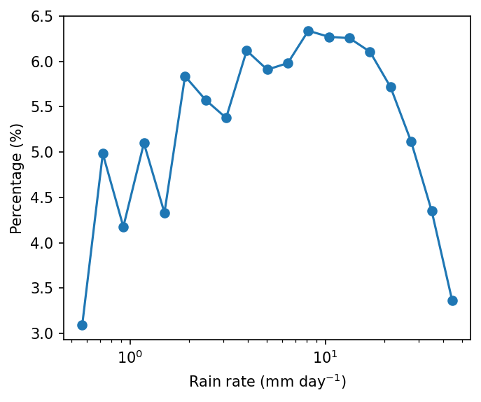
Example 2: 1-D probability distribution. Plot the probability distribution of daily precipitation rate.
Step 1: Read data.
pcp = xr.open_dataarray('./data/cmorph_sample.nc').sel(lat=slice(-15,15),lon=slice(90,160))
pcp_djf = pcp.sel(time=pcp.time.dt.month.isin([12,1,2]))
pcp_djf
<xarray.DataArray 'cmorph' (time: 2166, lat: 120, lon: 280)> Size: 291MB
[72777600 values with dtype=float32]
Coordinates:
  * time     (time) datetime64[ns] 17kB 1998-01-01 1998-01-02 ... 2021-12-31
  * lon      (lon) float32 1kB 90.12 90.38 90.62 90.88 ... 159.4 159.6 159.9
  * lat      (lat) float32 480B -14.88 -14.62 -14.38 ... 14.38 14.62 14.88
Attributes:
    standard_name:  lwe_precipitation_rate
    long_name:      precipitation
    units:          mm/day
    ver_note:       1998-2020: V1,0; 2021: V0.x.
comment: !!! CMORPH estimate is rainrate !!!Step 2: Count number of occurrence for each precipitation bin with flox. Technically, the precipitation is grouped by precipitation.
pdf = xarray_reduce(pcp_djf,
                    pcp_djf,
                    func='count',
                    isbin=True,
                    expected_groups=np.geomspace(0.5, 50, 20),
                    dim=['time','lat','lon'])
pdf_percent = pdf / pdf.sum() * 100.
pdf_percent
<xarray.DataArray 'cmorph' (cmorph_bins: 19)> Size: 152B
array([3.09464685, 4.98283472, 4.17693794, 5.09792383, 4.33013187,
       5.83681144, 5.57525959, 5.37691207, 6.11883881, 5.90911831,
       5.98125898, 6.33805064, 6.27095539, 6.25657   , 6.10623415,
       5.71656116, 5.11653848, 4.35264337, 3.36177241])
Coordinates:
* cmorph_bins (cmorph_bins) object 152B (0.5, 0.6371374928515668] ... (39....pcp_djfis the variable being grouped — we want to group precipitation valuesbyrain rate (the secondpcp_djf).func='count': Counts how many values fall into each bin (i.e., frequency of rainfall in each intensity range).isbin=True: Indicates that we want to group precipitation values into bins, not by exact values.expected_groups=np.geomspace(0.1, 50, 20): Defines the bin edges. Here we use logarithmic spacing (geomspace) from 0.1 mm to 50 mm, divided into 20 bins, because precipitation distribution is usually logarithmic scale.dim=['time','lat','lon']: Aggregates over all dimensions (time and space), so the result is a 1D histogram of rainfall intensity.
import matplotlib as mpl
from matplotlib import pyplot as plt

mpl.rcParams['figure.dpi'] = 150

fig, ax = plt.subplots(figsize=(5,4))
lineplt = pdf_percent.plot.line(x='cmorph_bins', marker='o', xscale='log',ax=ax)
ax.set_ylabel('Percentage (%)')
ax.set_xlabel(r'Rain rate (mm day$^{-1}$)')
Text(0.5, 0, 'Rain rate (mm day$^{-1}$)')
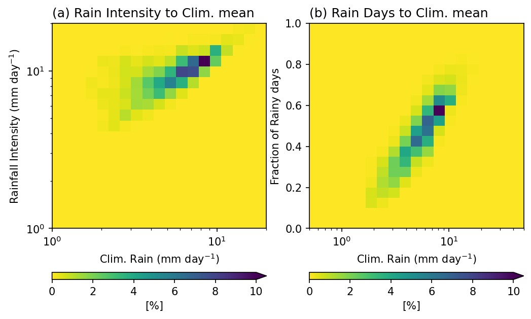
Example 3: 2-D Probability Distribution. Plot the 2-D probability distribution of annual mean rainfall, rainfall intensity, and fraction of rainy days (> 0.5 mm day \(^{-1}\) ).
These three metrics complement each other and provide a more complete picture of rainfall characteristics:
Annual mean rainfall (amount): the total rainfall, but it does not reveal whether it comes from frequent light rain or infrequent heavy rain.
Rainy days (frequency): shows how often it rains. High rainfall can result from many rainy days or from a few very wet days.
Rainfall intensity (amount per rainy day): distinguishes between light and heavy rain events.
Looking at these three variables together helps us understand how the total rainfall is distributed. This is important for interpreting climate regimes and hydrological impacts.
pcp_AnnualClm = pcp.mean(axis=0).rename('Annual_mean')
pcp_intensity = xr.where(pcp==0, np.nan, pcp).mean(axis=0,skipna=True).rename('Intensity')
                # Discard no precipitation points before averaing.
pcp_days = xr.where(pcp>0.5, 1, 0).mean(axis=0,skipna=True).rename('Rain_days')
           # Fraction of rainy days (> 0.5 mm day-1)
RI_Clm_pdf = xarray_reduce(pcp_intensity,
                           pcp_intensity,pcp_AnnualClm,
                           func='count',
                           dim=['lat','lon'],
                           isbin=(True,True),
                           expected_groups=(np.geomspace(1, 20, 20), np.geomspace(1, 20, 20)))
Days_Clm_pdf = xarray_reduce(pcp_days,
                             pcp_days,pcp_AnnualClm,
                             func='count',
                             dim=['lat','lon'],
                             isbin=(True,True),
                             expected_groups=(np.arange(0,1.05,0.05), np.geomspace(0.5, 50, 20)))
pcp_intensity(first argument): the variable passed to be reduced.pcp_intensity,pcp_AnnualClm: the two variables used for grouping. Flox will jointly bin data points according to rainfall intensity and annual mean rainfall.func='count': counts how many grid cells fall into each (intensity, annual rainfall) bin.dim=['lat','lon']: aggregation is applied over space to shape a histogram.isbin=(True,True): indicates both grouping variables are treated as binned quantities. The bins are based onexpected_groups: specifies the bin edges. Here both variables use log-spaced bins from 1 to 20 mm/day, which gives higher resolution at smaller values where rainfall tends to vary more strongly.
Note
The first argument pcp_intensity in this example, since func='count', is not used for its actual values**. It only provides shape and alignment for flox.
However, if the purpose is to calculate a statistic of another variable x conditioned on rainfall intensity and annual mean bins, then the first argument determines which variable is being aggregated. In that case, its values become meaningful for the computation.
Result:
RI_Clm_pdf is a 2D histogram showing how often certain combinations of rainfall intensity and annual mean rainfall occur across the spatial domain. This can be normalized to a probability distribution by dividing by the total count.
RI_Clm_pdf_percent   = RI_Clm_pdf / RI_Clm_pdf.sum() * 100.
Days_Clm_pdf_percent = Days_Clm_pdf / Days_Clm_pdf.sum() * 100.
mpl.rcParams['figure.dpi'] = 150

fig, axes = plt.subplots(1,2,figsize=(8,5))
ax = axes.flatten()

RI_Clm_plt = RI_Clm_pdf_percent.plot.pcolormesh(x='Annual_mean_bins',y='Intensity_bins',
                                                xscale='log',yscale='log',
                                                cmap='viridis_r',ax=ax[0],
                                                vmin=0, vmax=10,
                                                extend='max',
                                                cbar_kwargs={'orientation': 'horizontal', 'aspect': 30, 'label': r'[%]'})
ax[0].set_title('(a) Rain Intensity to Clim. mean',loc='left')
ax[0].set_ylabel(r'Rainfall Intensity (mm day$^{-1}$)')
ax[0].set_xlabel(r'Clim. Rain (mm day$^{-1}$)')

Day_Clm_plt = Days_Clm_pdf_percent.plot.pcolormesh(x='Annual_mean_bins',y='Rain_days_bins',
                                                   xscale='log',
                                                   cmap='viridis_r',ax=ax[1],
                                                   vmin=0, vmax=10,
                                                   extend='max',
                                                   cbar_kwargs={'orientation': 'horizontal', 'aspect': 30, 'label': r'[%]'})
ax[1].set_title('(b) Rain Days to Clim. mean',loc='left')
ax[1].set_ylabel('Fraction of Rainy days')
ax[1].set_xlabel(r'Clim. Rain (mm day$^{-1}$)')
Text(0.5, 0, 'Clim. Rain (mm day$^{-1}$)')
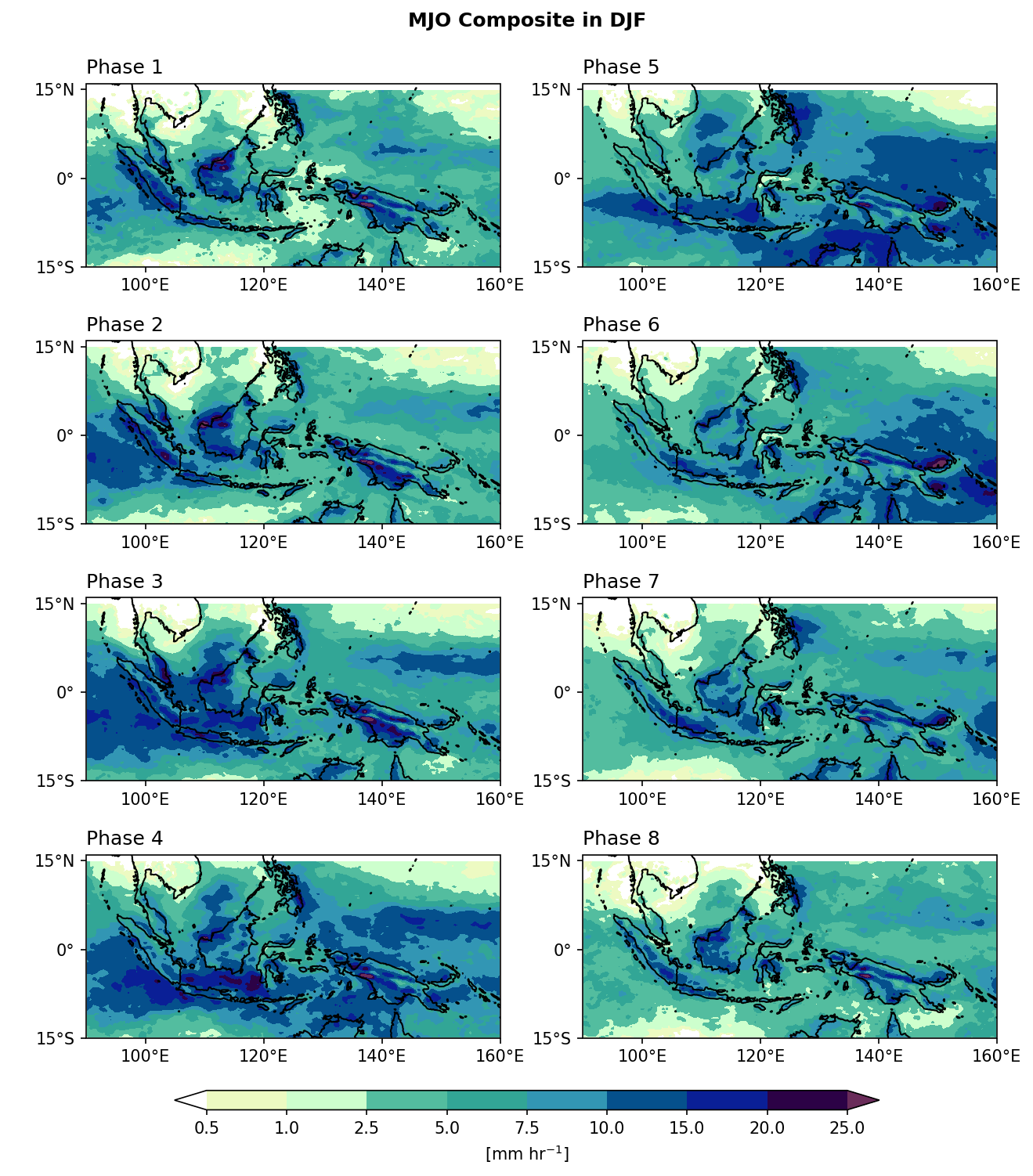
Example 4: Composite Mean. Plot rainfall composite mean for each MJO phase.
Step 1: Read MJO phase data from IRI data library.
import pandas as pd

# Read MJO data
mjo_ds = xr.open_dataset('http://iridl.ldeo.columbia.edu/SOURCES/.BoM/.MJO/.RMM/dods',
                         decode_times=False)

T = mjo_ds.T.values
mjo_ds['T'] = pd.date_range("1974-06-01", periods=len(T))  # Data starts from 1974-06-01

mjo_sig_phase = xr.where(mjo_ds.amplitude>=1,  mjo_ds.phase, 0).rename('mjo_phase')
                      # Only significant (amplitude >= 1) MJO events are preserved.

mjo_slice = mjo_sig_phase.sel(T=slice("1998-01-01","2021-12-31"))
mjo_djf = mjo_slice.sel(T=mjo_slice['T'].dt.month.isin([12, 1, 2])).rename({'T':'time'})
syntax error, unexpected WORD_WORD, expecting ';' or ','
context: Attributes { T { String calendar "standard"; Int32 expires 1755820800; String standard_name "time"; Float32 pointwidth 1.0; Int32 gridtype 0; String units "julian_day"; } amplitude { Int32 expires 1755820800; String units "unitless"; Float32 missing_value 9.99999962E35; } phase { Int32 expires 1755820800; String units "unitless"; Float32 missing_value 999.0; } RMM1 { Int32 expires 1755820800; String units "unitless"; Float32 missing_value 9.99999962E35; } RMM2 { Int32 expires 1755820800; String units "unitless"; Float32 missing_value 9.99999962E35; }NC_GLOBAL { String references "Wheeler_Hendon2004"; Int32 expires 1755820800; URL Wheeler and Hendon^ (2004) Monthly Weather Review article "http://journals.ametsoc.org/doi/abs/10.1175/1520-0493(2004)132%3C1917:AARMMI%3E2.0.CO;2"; String description "Real-time Multivariate MJO Index (with components of interannual variability removed)"; URL summary from BoM "http://www.bom.gov.au/climate/mjo/"; URL data source "http://www.bom.gov.au/climate/mjo/graphics/rmm.74toRealtime.txt"; String Conventions "IRIDL";}}
Illegal attribute
context: Attributes { T { String calendar "standard"; Int32 expires 1755820800; String standard_name "time"; Float32 pointwidth 1.0; Int32 gridtype 0; String units "julian_day"; } amplitude { Int32 expires 1755820800; String units "unitless"; Float32 missing_value 9.99999962E35; } phase { Int32 expires 1755820800; String units "unitless"; Float32 missing_value 999.0; } RMM1 { Int32 expires 1755820800; String units "unitless"; Float32 missing_value 9.99999962E35; } RMM2 { Int32 expires 1755820800; String units "unitless"; Float32 missing_value 9.99999962E35; }NC_GLOBAL { String references "Wheeler_Hendon2004"; Int32 expires 1755820800; URL Wheeler and Hendon^ (2004) Monthly Weather Review article "http://journals.ametsoc.org/doi/abs/10.1175/1520-0493(2004)132%3C1917:AARMMI%3E2.0.CO;2"; String description "Real-time Multivariate MJO Index (with components of interannual variability removed)"; URL summary from BoM "http://www.bom.gov.au/climate/mjo/"; URL data source "http://www.bom.gov.au/climate/mjo/graphics/rmm.74toRealtime.txt"; String Conventions "IRIDL";}}
Step 2: Group the precipitation data based on the MJO phase.
mjo_phase_comp = xarray_reduce(pcp_djf,
                               mjo_djf,
                               func='nanmean',
                               dim='time',
                               isbin=False,
                               )
mjo_phase_comp
<xarray.DataArray 'cmorph' (mjo_phase: 9, lat: 120, lon: 280)> Size: 1MB
array([[[1.5509361 , 1.5476524 , 1.5360179 , ..., 6.1897774 ,
         6.044517  , 5.838945  ],
        [1.644101  , 1.5174888 , 1.6073403 , ..., 6.6764784 ,
         6.6883655 , 6.3710103 ],
        [1.7099406 , 1.5615454 , 1.6053046 , ..., 7.1074147 ,
         7.0514264 , 6.989376  ],
        ...,
        [1.2247697 , 1.2321248 , 1.0660772 , ..., 0.9790045 ,
         0.91200596, 0.8479941 ],
        [0.9963893 , 0.90916795, 0.7632095 , ..., 1.0414264 ,
         0.996211  , 0.9376969 ],
        [0.74106985, 0.6703715 , 0.6609807 , ..., 1.0852897 ,
         1.0059881 , 0.92294204]],

       [[2.1850576 , 2.1586208 , 2.3988507 , ..., 5.4770117 ,
         4.7149425 , 4.7413793 ],
        [2.2839081 , 2.4195402 , 2.4873564 , ..., 5.5850577 ,
         4.9080462 , 5.1747127 ],
        [2.4034483 , 3.0367815 , 3.254023  , ..., 5.462069  ,
         5.521839  , 5.8977013 ],
...
        [0.2897544 , 0.26273686, 0.29249123, ..., 0.74992985,
         0.7251579 , 0.681193  ],
        [0.24196492, 0.19701755, 0.1731579 , ..., 0.7130176 ,
         0.6249825 , 0.6207018 ],
        [0.16712281, 0.14017543, 0.15249123, ..., 0.62736845,
         0.57480705, 0.5857895 ]],

       [[1.9496454 , 1.8248227 , 1.8163121 , ..., 4.546099  ,
         4.824823  , 5.4425535 ],
        [1.9907802 , 2.1276596 , 2.283688  , ..., 4.7184396 ,
         5.012766  , 5.05461   ],
        [2.555319  , 2.703546  , 2.8758867 , ..., 5.4425535 ,
         5.6014185 , 5.35461   ],
        ...,
        [0.75886524, 0.72269505, 0.57588655, ..., 3.2198582 ,
         3.0680852 , 3.1226952 ],
        [0.8056738 , 0.6815603 , 0.55602837, ..., 3.7794328 ,
         3.487234  , 3.0744681 ],
        [0.5156028 , 0.56950355, 0.5382979 , ..., 3.7475178 ,
         3.7709222 , 3.3829787 ]]], dtype=float32)
Coordinates:
  * lon        (lon) float32 1kB 90.12 90.38 90.62 90.88 ... 159.4 159.6 159.9
  * lat        (lat) float32 480B -14.88 -14.62 -14.38 ... 14.38 14.62 14.88
  * mjo_phase  (mjo_phase) float32 36B 0.0 1.0 2.0 3.0 4.0 5.0 6.0 7.0 8.0
Attributes:
    standard_name:  lwe_precipitation_rate
    long_name:      precipitation
    units:          mm/day
    ver_note:       1998-2020: V1,0; 2021: V0.x.
comment: !!! CMORPH estimate is rainrate !!!In this example, precipitation data
pcp_djfis grouped by each MJO phasemjo_djf. For each MJO phase group,func='nanmean'calculates the mean precipitation over time dimension (dim='time'). That is, all time steps belonging to the same MJO phase are averaged together.isbin=False: Means we are grouping by the exact values ofmjo_djf(the phase categories 1–8), not by bins.
Step 3: Plotting.
import cmaps
from cartopy import crs as ccrs
from cartopy.mpl.gridliner import LONGITUDE_FORMATTER, LATITUDE_FORMATTER

mpl.rcParams['figure.dpi'] = 150

fig, axes = plt.subplots(4,2,
                         subplot_kw={'projection': ccrs.PlateCarree()},
                         figsize=(10,11))
ax = axes.flatten()
lon_formatter = LONGITUDE_FORMATTER
lat_formatter = LATITUDE_FORMATTER

clevs = [0.5,1,2.5,5,7.5,10,15,20,25]

porder = [0,2,4,6,1,3,5,7]

for i in range(1,9):
    cf = (mjo_phase_comp[i,:,:].plot.contourf(x='lon',y='lat', ax=ax[porder[i-1]],
                                         levels=clevs,
                                         add_colorbar=False,
                                         cmap=cmaps.precip_11lev,
                                         extend='both',
                                         transform=ccrs.PlateCarree()))
    ax[porder[i-1]].coastlines()
    ax[porder[i-1]].set_extent([90,160,-15,16],crs=ccrs.PlateCarree())
    ax[porder[i-1]].set_xticks(np.arange(100,180,20), crs=ccrs.PlateCarree())
    ax[porder[i-1]].set_yticks(np.arange(-15,30,15), crs=ccrs.PlateCarree())   # 設定x, y座標的範圍,以及多少經緯度繪製刻度。
    ax[porder[i-1]].xaxis.set_major_formatter(lon_formatter)
    ax[porder[i-1]].yaxis.set_major_formatter(lat_formatter)
    ax[porder[i-1]].set_xlabel(' ')
    ax[porder[i-1]].set_ylabel(' ')
    ax[porder[i-1]].set_title(' ')
    ax[porder[i-1]].set_title('Phase '+str(i), loc='left')

# Add a colorbar axis at the bottom of the graph
cbar_ax = fig.add_axes([0.2, 0.07, 0.6, 0.015])
# Draw the colorbar 將colorbar畫在cbar_ax這個軸上。
cbar = fig.colorbar(cf, cax=cbar_ax,
                    orientation='horizontal',
                    ticks=clevs,
                    label=r'[mm hr$^{-1}$]')

plt.subplots_adjust(hspace=0.15)
plt.suptitle('MJO Composite in DJF',y=0.92,size='large',weight='bold')
plt.show()